MainPage:Nuclear:Summer2019:PWO
Lead Tungstate Crystal 3D Mapping
Summary
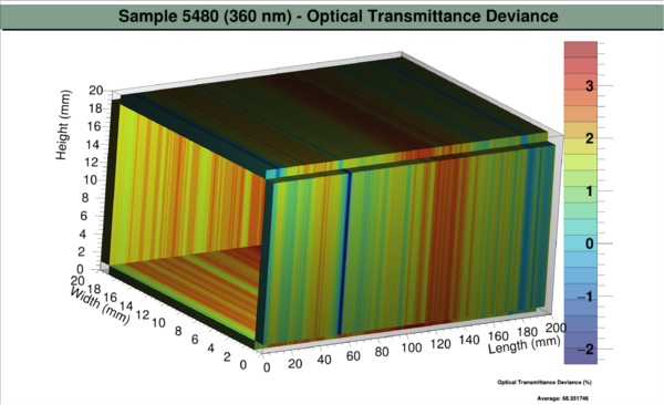
Since crystals are grown, there are imperfections in the quality of crystals. To check the quality of each crystal, transverse optical transmittance measurements are taken. To represent the resulting data, a 3D map was developed through CERN’s ROOT. This application allows the user to easily identify sub-standard crystals and locate imperfections within the crystal.
Introduction
Lead tungstate (PWO) crystals act as scintillators in electromagnetic calorimeters. This type of calorimeter measures the energy of particles that interact via the electromagnetic force (Bock).
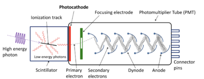
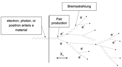
As seen in Figure 1, when a high-energy photon, electron, or positron enters the PWO crystal, it scintillates and produces photons. Figure 2 breaks down the process of scintillation and how a electromagnetic showers occurs. The high-energy incoming particle causes pair production which results in an electron and positron. As the electron and positron travels through the particle, Bremsstrahlung (energy losses as a charged particle accelerates around a nucleus) occurs and photons are emitted. These photons can cause another cycle of pair production and Bremsstrahlung until all the energy has been deposited into the crystal (Landau and Rummer).
Next, in figure 1, the photomultiplier tube converts incident photons into a signal. Specifically, these photons interact with a photocathode which produces electrons through the photoelectric effect. However, this signal is too weak to detect, so it must be amplified. The primary electron is directed by a magnetic field towards a dynode. When the primary electron interacts with the dynode, it creates multiple secondary electrons which travel to another dynode for further amplification. Eventually, a signal can be detected and the operator can measure the energy of the incoming particle (Glenn).
Additionally, lead tungstate is ideal as a scintillator in a compact electromagnetic calorimeter due to the following properties: high density (8.3 g/cm3), short radiation length (0.89 cm), small Moliere radius (2.2 cm), and fast scintillation time (80% in 25ns) (CMS Physics Technical Design Report). Despite this, the manufacturing process of crystals are yet to be perfected. As seen in the following sections, there can be significant variations in the transverse optical transmittance of these crystals. Thus, it’s important to select high-quality crystals. Developing a 3D map would allow easier identification of imperfections in the crystal because the user could visually identify and locate the imperfections.
Method
Crystal Preparation
Each lead tungstate crystal was thorougly cleaned with 70% isopropyl alcohol and dried with a Kimwipes. Also, temporarily remove the label as it interferes with the measurement. Although the crystal are dense, they are very brittle and easy to chip. Be sure to handle with care and use gloves at all times.
Lambda 950 Spectrophotometer
The transverse optical transmittance of each crystal was measured using the Lambda 950 Spectrophotometer. An apparatus with a stepper motor was installed to slide the crytal along its longitudinal axis. The stepper motor moved 1 mm per second. At the start of calibration and every trial, the whole apparatus was covered in a black cloth to prevent any light from entering into the chamber. The optical transmittance was auto-zeroed after changing each wavelength and the iris was set to 2.0 mm. Usually, the the wavelength 360 nm was used as it created higher amounts of deviance to allow easier identification of imperfections.
Crystal Orientation
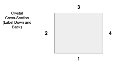
Place the end of the crystal with the (now removed) label in the back. As seen in the diagram, side 1 is with the label down.
Data Processing
Open the *.csv files with Microsoft Excel. For a plot or 2D map, delete the column with time and cut the optical transmittance measurements. Usually, the cut optical transmittance measurement should vary by 2% on the ends. Then, save the spreadsheet as a tab-delimited text file. To input the data into the application, don't forget to change the name of the file it reads in.
Application Development
ROOT
Developed by CERN, ROOT is an object-oriented program and library that is designed to efficiently handle large amounts of data. As of August 2019, it is written in C++.
Recommended Resources for Beginners (as of ROOT 6.18.0 )
- Google!
- ROOT YouTube Tutorial
- ROOT Primer
Simple Plot
{
    g = new TGraph("Sample72_1.txt"); // Reads data from a .txt file. CHANGE AS NEEDED
    g->SetMinimum(0);
    g->SetMaximum(100);
    g->GetXaxis()->SetLimits(0, 200);
    g->SetTitle("Sample 72 - Position vs Transverse Optical Transmittance; Position (mm); Optical Transmittance (%)");
    g->SetMarkerStyle(7);
    g->Draw("ALP");
}
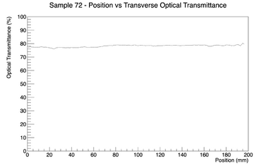
The .txt files have one column of transverse optical transmittance data and are stored in the tab-delimited text file format. This .txt file was made from Microsoft Excel and cut at the edges.
2D Map
TCanvas *th2polyBoxes()

#include <fstream>
#include <iostream>
#include <stdio.h>
#include <fstream>


void Crystal72_2D_2(){

  struct input_t

  //Define array  structure for input

  {
    Double_t transmittance;
  };

  input_t input;

  // Reads data from ONE column of data

  FILE *f = fopen("Crystal5478_620.txt","r"); // Reads data from a .txt file. CHANGE AS NEEDED
  char line[400];

  // Creates array

  Double_t transArray[196];


  Int_t j=0;
  TFile *file = new TFile("test.root","RECREATE");
  for(Int_t i;fgets(&line[0],500,f);i++){
    if (line[0] == '#'){
      continue;
    }else{
      sscanf(&line[0], "%lf", &input.transmittance);
    }

      transArray[j]=input.transmittance;
      j++;

   }


  //Finds the average
  float avg = 0.0;
  float sum = 0.0;
  int size;

  size = sizeof(transArray) / sizeof(transArray[j]);

  for (int i = 0; i < size; ++i)
   {
   sum += transArray[i];
  }
  avg = ((float)sum)/size; //or cast sum to double before division

  cout << "Average  " << avg << "\n";

  // Calcuates deviance

  Double_t dev[size];

  for(int i = 0; i < size-1; i ++)
  {
      dev[i]= transArray[i] - avg;
      //cout << "Deviance  " << dev[i] << "\n";
  }


  //Set-up canvas/graph

  TCanvas *ch2p2 = new TCanvas("ch2p2","ch2p2",1435,415);
  gStyle->SetPalette(kRainBow);
  TH2Poly *h2p = new TH2Poly();
  h2p->SetName("Boxes");
  h2p->SetTitle("Boxes");
  Int_t i,l;
  Int_t nx = size;
  Int_t ny = 1;
  Double_t xval1,yval1,xval2,yval2;
  Double_t dx=1, dy=4;
  xval1 = .5;
  xval2 = dx + xval1;
  yval1 = -4;
  yval2 = dy;

  // In the x, there is a bin per mm.
  // In the y, there is only one bin. In this sense, "y" is meaningless.
  // Optical transmittance is reflected in the z.


  // This "for" loop adds "nx" bins in increments of "dx".
  for (i = 0; i<nx; i++) {
     h2p->AddBin(xval1, yval1, xval2, yval2);
     xval1 = xval2;
     xval2 = xval2+(dx);

     //Since y is meaningless, the weight is used to create the different shades of color

     h2p->Fill(i, .1 , dev[i]);
  }

  // Sets the range and removes the y-axis.

  h2p->GetXaxis()->SetRangeUser(0,200);
  h2p->GetYaxis()->SetRangeUser(0,100);
  h2p->GetZaxis()->SetRangeUser(-3,3);
  h2p->GetYaxis()->SetLabelOffset(999);
  h2p->GetYaxis()->SetLabelSize(0);


  // Sets the title, removes the stats box, and draws graph.
  h2p->SetTitle("Crystal5476 (360 nm) - Position vs Deviance in Optical Transmittance; Position(mm); ;Optical Transmittance Deviance(%)");
  h2p->GetZaxis()->SetTitleOffset(0.5);
  h2p->SetStats(0);
  h2p->Draw("COLZ");

  return ch2p2;
}
3D Map
namespace {

Double_t my_transfer_function(const Double_t *x, const Double_t * /*param*/)
{

  if (*x>-.0001 && *x<.0001)
      return 0.001;
   return 1.;
}
}

void glgraph(){

int data = 0;

// Reads data in

ifstream file { "5608.txt" }; // Reads data from a .txt file. CHANGE AS NEEDED
if (!file.is_open()) return -1;

double transArray [200][4]{};

for (int i{}; i != 200; ++i) {
    for (int j{}; j != 4; ++j) {
        file >> transArray[i][j];

    }
}


  // Calculates the average
  float avg = 0.0;
  float sum = 0.0;
  int size;

  for (int i{}; i != 200; ++i) {
    for (int j{}; j != 4; ++j) {
    size = sizeof(transArray) / sizeof(transArray[i][j]
 );
  sum += transArray[i][j];
    }
  }
  avg = ((float)sum)/size;

  double dev[size][4];

  cout << "Average Optical Transmittance  " << avg << "\n";

  char average[64];
  int ret = snprintf(average, sizeof average, "%f", avg);

if (ret < 0) {
    return EXIT_FAILURE;
}
if (ret >= sizeof average) {
    //Result was truncated - resize the buffer and retry.
}

// Calculate deviance and stores it into an array

 for (int i{}; i != 195; ++i) {
    for (int j{}; j != 4; ++j) {
      dev[i][j]= transArray[i][j] - avg;
    }}

// Sets the parameters for the 3D map

 TH3F *hist = new TH3F("glvoxel", "OT", (size/4), 0., (size/4), 20, 0., 20., 20, 0., 20.);

   for (UInt_t i = 0; i < 200; ++i) {
     for (Int_t j = 1; j< 19;j++){
       hist->Fill(i, j, 0., dev[i][0]); //Side 1
       hist->Fill(i, 19.9, j, dev[i][1]); //Side 2
       hist->Fill(i, j, 19.9, dev[i][2]); // Side 3
       hist->Fill(i, 0.1,j , dev[i][3]); // Side 4
       }
    }


   gStyle->SetCanvasPreferGL(1);
   hist->Draw("glcolz");

// Label and set ranges for x-axis, y-axis, and z-axis
   hist->GetXaxis()->SetTitle("Length (mm)");
   hist->GetXaxis()->SetTitleOffset(1.5);
   hist->GetYaxis()->SetTitle("Width (mm)");
   hist->GetYaxis()->SetTitleOffset(1.5);
   hist->GetZaxis()->SetTitle("Height (mm)");
   hist->GetZaxis()->SetTitleOffset(1.5);
   hist->GetZaxis()->SetRangeUser(-10,0);

   hist->SetTitle("OT");
   gStyle->SetCanvasPreferGL(1);
   gStyle->SetPalette(kRainBow);
   hist->SetFillColor(9);
   hist->Draw("glcolz");

// Creates the title for the 3D map
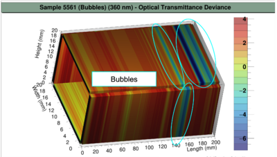
   TPaveLabel *title = new TPaveLabel(-1., 0.86, 1., 0.98, "Sample 5608 (Bubbles) (360 nm) - Optical Transmittance Deviance");

   TLatex *tex = new TLatex(0.75,0.05,"Optical Transmittance Deviance (%)");
  tex->SetNDC();
  tex->SetTextSize(.015);
  tex->SetLineWidth(2);
  tex->Draw();
  title->SetFillColor(32);
  title->Draw();


// Outputs the average
  TLatex *avg3 = new TLatex(0.81, 0.01, TString::Format("Average: %s", average));
  avg3->SetNDC();
  avg3->SetTextSize(.015);
  avg3->SetLineWidth(2);
  avg3->Draw();
  title->SetFillColor(32);
  title->Draw();

   //Now, specify the transfer function.
   TList * lf = hist->GetListOfFunctions();
   if (lf) {
      TF1 * tf = new TF1("TransferFunction", my_transfer_function);
      lf->Add(tf);
   }
}
The .txt files is similar to the ones from the 2D map except it has 4 columns. Each position is linked to the column number according to the following figure. Position 1 is with the label down.
Data Analysis
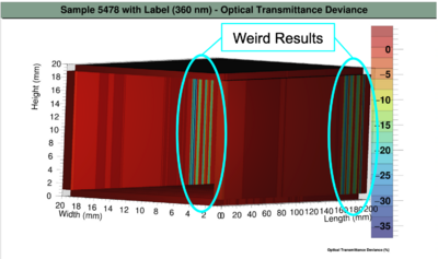
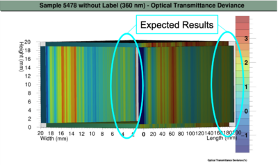
Crystal 5478 (Label Interference)
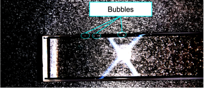
Crystal 5561 (Bubbles)
Crystal 5609 (Chipped)
Crystal 5480 (Fingerprint)
Conclusion
Unlike longitudinal measurements which only record one area, the transverse transmittance measures along the length of the crystal. Thus, with the 3D map, one could more accurately identify and locate imperfections such as bubbles and chips in the crystal. Furthermore, the interference of items such as fingerprints and labels underlined the importance of thoroughly cleaning the crystal. However, the 3D map system is limited in the transverse transmittance measurements only takes data on axis. As an extension, one could develop a system to measure off-axis, which would increase the resolution of the 3D map to pick-up smaller imperfections.
Presentations
Other Projects
KaonLT - Stacking Histograms
Overview: The KaonLT experiment takes measurements of the L/T separated kaon electroproduction cross section. These measurement are important to ehance our understanding of the kaon's structure.
Purpose: After receiving data, cuts are made. To compare the cuts, an application needs to be developed to graph the pre-cut and post-cut data on the same histogram. Additionally, since data is stored in a tree, the program must identify the correct user-selected leaf from each root file.
In the attached sample file, the user only applied cuts to the TDCTimeRaw plots. Applying cuts to the TDCTimeRaw plots affects the TDCTime plots. TDCTime plots only shows accepatable physics coincidence events, so TDCTimeRaw and TDCTime plots should differ slightly.
//Modified script from Richard Trotta.
#include <string>
#include <cstdio>
#include <iostream>


void plot_Stat2(Int_t runNum = 4889, Int_t numEvts = 0, TString leaf = ""){

   if(runNum==0){

  	cout << "Please enter run number ...\n";
  	cin >> runNum;
	}

   /* if(numEvts==0){

  	cout << "Please enter number of events in replay ...\n";
  	cin >> numEvts;
	}*/

   if(leaf==""){

  	cout << "Please pick a leaf ...\n";
  	cin >> leaf;
	}

    TString rootfile1 = Form("/Applications/root_v6.18.00/macros/Overlap/coin_replay_production_%i_cut", runNum);

  TString outputhist1;
  outputhist1 = rootfile1 + ".root";

  TString outputpdf1;
  outputpdf1 =  Form("OUTPUT/statsPlots_%i.pdf",runNum);

  TFile *f1 = TFile::Open(outputhist1);
  if( !f1 || f1->IsZombie()){
	return;
  }

  TString rootfile2 = Form("/Applications/root_v6.18.00/macros/Overlap/coin_replay_production_%i_nocut", runNum);

  TString outputhist2;
  outputhist2 = rootfile2 + ".root";

  TString outputpdf2;
  outputpdf2 =  Form("OUTPUT/statsPlots_%i.pdf",runNum);

  TFile *f2 = TFile::Open(outputhist2);
  if( !f2 || f2->IsZombie()){
	return;
  }

  TString cutLeaf, nocutLeaf, deltaLeaf,xptarLeaf, yptarLeaf, wLeaf;

  TTreeReader r("T", f1);
  TTreeReader n("T", f2);

  TCanvas *c1 = new TCanvas("c1","Stat plots", 600, 400);
  // TCanvas *c2 = new TCanvas("c2","Stat plots", 600, 400);
  //TCanvas *c3 = new TCanvas("c3","Stat plots", 600, 400);
  //TCanvas *c4 = new TCanvas("c4","Stat plots", 600, 400);

  TH1F *h1 = new TH1F("h1", Form("Run %i ; T.coin.pDCREF1_tdcTimeRaw", runNum), 500,15200,16600);
  // TH1F *h1 = new TH1F("h1", Form("Run %i - Uncut(Blue) vs Cut(Red); %s", runNum, leaf), 300,200,500);
  //TH2F *h2= new TH2F("h2","Xptar vs Yptar", 200, -0.1, 0.1,200,-0.1, 0.1);
  //TH2F *h3= new TH2F("h3","W^2 vs Xptar ", 200, -.1, .1,200,0, 20);
  //TH2F *h4= new TH2F("h4","W^2 vs Yptar ", 200, -.1, .1,200,0, 20);

  TH1F *h2 = new TH1F("h2","Uncut", 500,15200,17000);

  //if(spec == "hms"){
  cutLeaf = leaf;
  nocutLeaf = leaf;
  /* xptarLeaf = "H.gtr.th";
    yptarLeaf = "H.gtr.ph";
    //deltaLeaf = "H.gtr.dp";
    wLeaf = "H.kin.W2";*/
     TTreeReaderValue<Double_t> cut(r, cutLeaf);
     TTreeReaderValue<Double_t> nocut(n, nocutLeaf);
     /* TTreeReaderValue<Double_t> yfp(r, yfpLeaf);
  TTreeReaderValue<Double_t> xptar(r, xptarLeaf);
  TTreeReaderValue<Double_t> yptar(r, yptarLeaf);
  TTreeReaderValue<Double_t> invmass(r, wLeaf);*/
     //TTreeReaderValue<Double_t> hsdelta(r,deltaLeaf);
   while(r.Next()){

     /*int k;
     cout << "While loop W^2 " << k << '\n';
      if(*hsdelta > -8 && *hsdelta < 8
	){*/

     h1->Fill(*cut);
	//h2->Fill(*yptar,*xptar);
	//h3->Fill(*xptar,*invmass);
	//h4->Fill(*yptar,*invmass);

	/*	k++;
		}*/

       }

   h1->Draw();
   h1->SetLineColor(kMagenta);
   h1->SetLineWidth(2);

  while(n.Next()){

    /*int k;
     cout << "While loop W^2 " << k << '\n';
      if(*hsdelta > -8 && *hsdelta < 8
	){*/

	h2->Fill(*nocut);
	//h2->Fill(*yptar,*xptar);
	//h3->Fill(*xptar,*invmass);
	//h4->Fill(*yptar,*invmass);

	/*	k++;
		}*/

       }
   //h1->GetXaxis()->SetTitle("yfp");
   //h1->GetYaxis()->SetTitle("");

  //h2->GetXaxis()->SetTitle("yptar");
    //h2->GetYaxis()->SetTitle("xptar");

  //h3->GetYaxis()->SetTitle("W^2");
  //h3->GetXaxis()->SetTitle("xptar");

  //h4->GetYaxis()->SetTitle("W^2");
  //h4->GetXaxis()->SetTitle("yptar");

  //c1->Divide(2,2);
  //c1->cd(1);
  gStyle->SetOptStat(0);
  h2->SetLineColor(kBlue+4);
  h2->SetLineWidth(2);
  h2->Draw("SAME");
  //h1->SetStats(1111)

   auto legend = new TLegend(0.8,0.8,0.9,0.9);
   legend->SetHeader("Legend","C"); // option "C" allows to center the header
   legend->AddEntry("h1","Cuts","l");
   legend->AddEntry("h2","No cuts","l");
   legend->Draw();

  //c1->Print(outputpdf1+"(");
  //c1->cd(2);
  //h2->Draw("Colz");
  //c2->Print(outputpdf+ ")");
  //c1->cd(3);
  //h3->Draw("Colz");
  //c3->Print(outputpdf);
  //c1->cd(4);
  //h4->Draw("Colz");
  //c4->Print(outputpdf+")");

  //c1->Print("OUTPUT/pngFiles" + spec + "_statsPlots_" + Form("%i",(int)runNum) + ".png");

  /*const string sep = " |";
  const int total_width = 154;
  const string line = sep+ string(total_width-1,'-') + '|';

  ofstream myfile;*/


  /*if(spec=="shms"){
    xfpLeaf = "P.dc.x_fp";
    yfpLeaf = "P.dc.y_fp";
    xptarLeaf = "P.gtr.th";
    yptarLeaf = "P.gtr.ph";
    deltaLeaf = "P.gtr.dp";
  TTreeReaderValue<Double_t> xfp(r, xfpLeaf);
  TTreeReaderValue<Double_t> yfp(r, yfpLeaf);
  TTreeReaderValue<Double_t> xptar(r, xptarLeaf);
  TTreeReaderValue<Double_t> yptar(r, yptarLeaf);
  TTreeReaderValue<Double_t> invmass(r, wLeaf);
  TTreeReaderValue<Double_t> ssdelta(r,deltaLeaf);
    while(r.Next()){

      int k;
      cout << "While loop W^2 " << k << '\n';

      if(*ssdelta > -10 && *ssdelta < 15
	 ){

	h1->Fill(*yfp,*xfp);
	//h2->Fill(*yptar,*xptar);

	k++;
      }

      }*/

  //h1->GetXaxis()->SetTitle("yfp");
  //h1->GetYaxis()->SetTitle("xfp");

  //h2->GetXaxis()->SetTitle("yptar");
  //h2->GetYaxis()->SetTitle("xptar");

  //h3->GetYaxis()->SetTitle("W^2");
  //h3->GetXaxis()->SetTitle("xptar");

  //h4->GetYaxis()->SetTitle("W^2");
  //h4->GetXaxis()->SetTitle("yptar");

  //c1->Divide(2,2);
  //c1->cd(1);
  //c1->Print(outputpdf+"");
  //c1->cd(2);
  //h2->Draw("Colz");
  //c2->Print(outputpdf+ ")");
  //c1->cd(3);
  //h3->Draw("Colz");
  //c3->Print(outputpdf);
  //c1->cd(4);
  //h4->Draw("Colz");
  //c4->Print(outputpdf+")");

  c1->Print(Form("/Applications/root_v6.18.00/macros/Overlap/Output/statsPlots_%i_.pdf",(int)runNum));

  /*const string sep = " |";
  const int total_width = 154;
  const string line = sep+ string(total_width-1,'-') + '|';

  ofstream myfile;
  }*/


}
Sample Files - Stacking Histograms
Works Cited
Bock, Rudolf K. “Calorimeter.” Calorimeter , CERN, 9 Sept. 1998, <http://web.archive.org/web/20071220021724/http://rd11.web.cern.ch/RD11/rkb/PH14pp/node19.html>.
CMS Physics Technical Design Report. CERN, 2006, CMS Physics Technical Design Report.
Glenn F Knoll. Radiation Detection and Measurement, Third Edition 2000. John Wiley and Sons , ISBN 0-471-07338-5
Landau, Lev Davydovitch, and G. Rumer. “The Cascade Theory of Electronic Showers.” The Royal Society of Mathematical, Physical, and Engineering Sciences , 18 Nov. 1937.
