MainPage:Nuclear:Summer2016:12GeVExp

Elastic Analysis, at CUA

File:123.pdf

Abstract

Previously, scientists believed pions and kaons, particles that constitute matter, were points without structure. With new research that theory has been proven incorrect. Next year Catholic University of America at Jefferson Lab will conduct a kaon experiment. The goal being to detect kaons with the Gas Cherenkov Detector of the High Momentum Spectrometer (HMS). The HMS measures the particles scattered by the electron when it hits the target proton. With this particle detection they hope detect, predict, and study the kaon particle’s form factor. In Addition, the experiment can be set up to detect both kaons and pions. This preferred set up that detects both kaons and pions will allow the researchers to study the Pion’s form factor as well. In order for both particles to be studied, the experiment must be optimized and set up correctly. To optimize the experiment code was typed and data analysis was used to determine the proper set up. Once, a simulation was run using previous data collected from a similar experiment at the Jefferson Lab. Then the total number of events from the similar experiment and simulation were plotted onto a histogram. Code was written in root that normalized and cut both data sets allowing them to be compared. The normalized data confirmed that the number of events was equal to the number of electrons sent or the actual yield. By studying the graphs insight into which aspects of the experiment to be done next year were optimized could be instituted such as different materials, angels, or methods. By detecting both sub atomic particles the experiment had the best chance to discover each particles form factor.

Personal Contribution Statement

During my summer internship with CUA (Catholic University of America) I ran simulations from previous trials. I then graphed the simulations with the previous results on a histogram. I tested and created code through CERN’s root program that normalized and cut the histograms. This allowed for it to be compared. It also confirmed the actual yield where the input equals the output. The comparison also allowed me to suggest where improvements could have been made by looking at where certain data was different than predicted. I helped to optimize the set up to best detect both kaons and pions.

Validating the Simulation with Previous Elastic data from Hall C

First I began by validating a Monte Carlo simulation, which is used to predict the probability of certain outcomes of events. The monte Carlo simulation is used to predict the scattering of particles. The simulation needed to be validated because it would then be used to make predictions for a kaon experiment to be done next year. Since the Kaon experiment is completely theoretical, the simulation needed to be validated to give an accurate number of kaons and pions. Without an accurate number we would not be able to predict whether or not we could have insights into the pion form factor.

To validate the simulation, first, four input forms were created to mimic previously completed elastic scattering experiments from JLab. The simulation was set up to track the scattered electron which is fed into the HMS (High Momentum Spectrometer). The experiment also tracks the scattered electron. By comparing the data collected from the experiment and simulation we can determine whether the simulation is accurate enough to be used to make predictions for the kaon experiment.

Particle detection

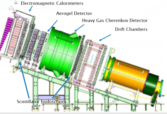
Various particles can be detected in the HMS and SHMS (Super High Momentum Spectrometer).

fig 1:

Shown above are the particle identification detectors within the spectrometers. To detect electrons use: gas Cherenkov detector and the electromagnetic calorimeter. For Kaon and Pion detection use: the Heavy Gas Cherenkov and the Aerogel Detector. The other detectors such as the Drift Chambers are used for particle trajectories, whereas the scintillator hodoscopes are used for for timing.

Table 1:

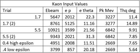
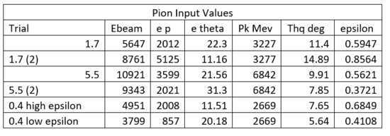
The various input values are shown above. By changing the election momentum and angle, we can better learn our spectrometer. We can also compare the results of the experiment and simulation at each setting to make sure the simulation accurately models the data.

Preliminary Results: shown below is a graph containing the simulations result superposed with the experimental recorded data.

The Graph above only contains weights, normfac, and the prescale. The normfac accounts for the proper cross section. The prescale is needed because the computers can only pick up so many particles at once. Instead, it will measure for example one particle for every eighty that pass through to avoid crashing. Therefore the experimental data must be multiplied by eighty in this case to get the actual amount of data points that went through the detector. No cuts have been applied to the simulation's data.

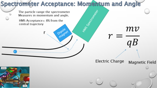
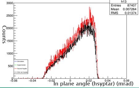
Next cuts needed to be applied to the simulation. The HMS can only accept a particle within certain ranges. The ranges are the hsxptar, hsyptar, and the hsdelta. The hsxptar (out of plane angle) contains the horizontal plane angle acceptance that the electron follows as it heads into the spectrometer. The cut for hsxptar is plus or minus .09 mrad from the center path(better phrase needed). The hsyptar (in plane angle) is the vertical planar acceptance into the spectrometer. The hsyptar acceptance is plus or minus 0.024 mrad from the center path(still better phrase). Finally, the electron must be bent into the the HMS. This is the hsdelta cut.

fig 1:

Shown below is the formula for the hsdelta cut. The particle acceptance depends on the particles momentum. r represents the radius of the curve that the electron is bent around into the spectrometer. The spectrometer acceptance is plus or minus 8% from the center curve.

Cuts are applied to the simulation data because without them every particle is accepted. The cuts must be applied to take into account what the spectrometers at JLab accept to get the most accurate simulation of what will occur. The process of cutting removes the data points which fall outside of the specified spectrometer acceptance.

Graph 2:

Shown above is the hsyptar data with cuts applied. The two data sets are very similar, in which with cuts applied both are accepting very similar amounts of particles.

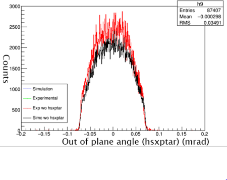
Graph 3:

Shown above is the hsxptar data with cuts applied. The two data sets are very similar, in which with cuts applied both are accepting very similar amounts of particles.

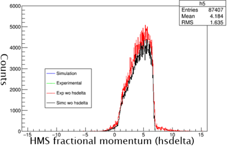
Graph 4:

Shown above is the hsdelta with cuts applied. The two data sets are very similar, in which with cuts applied both are accepting very similar amounts of particles.

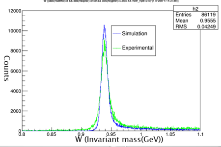
Graph 5:

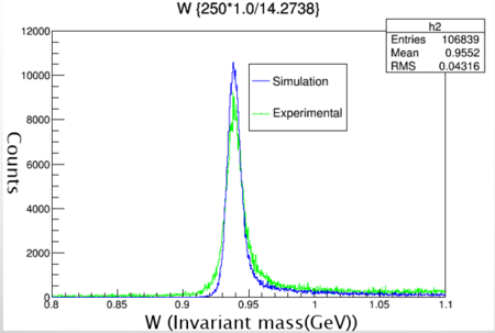
Shown above is a histogram with W (invariant mass) plotted from the 47339 trial. The peak should be at the GeV of a proton 0.94 which it is. This means the simulation has gone correctly so far.

Particle Detection (Calorimeter and Gas Cherenkov Detector)

Both the detectors detect electrons. The Heavy Gas Cherenkov Detector contains a heavy gas on the inside. The electron passes through the gas faster than the speed light does. In turn, the particle gives off Cerenkov radiation (Blue light) which is picked up by the detector and measured in photo electrons. The Calorimeter works by measuring the particle's energy as it passes through the detector.

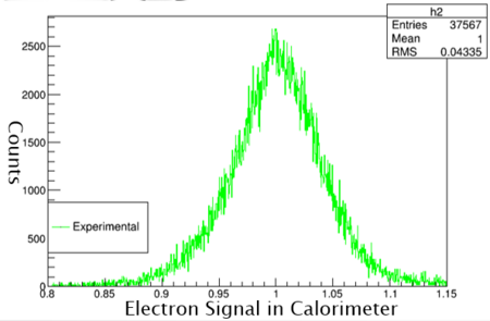
Graph 5:

Shown above are the readings from the Calorimeter. Since there is only a single peak at 1 and no other peaks no other particles other than the electron are being detected.

Graph 6:

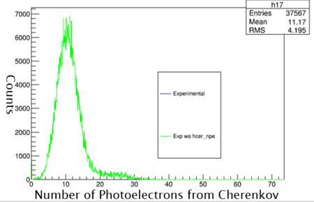
Shown above is the number of counts for each number of photo electrons. One electron emits ten photo electrons in the Gas Cherenkov Detector. Since only electrons are being detected there is no cross contamination from pions or other sub-atomic particles.

Validation

After applying all of the cuts and determining there was no cross contamination we progressed onto validating the simulation. In order to do so we divided the experimental yield by the simc yield. Theoretically we would get one if the simulation was the same as the experiment. To determine the statistical uncertainty we used a poisson distribution.

fig 2:

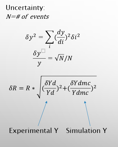
Shown above is the uncertainty formula used. The derivative for the simulation and experiment simplifies to the square root of the number of events divided by the number of events. Then those number are squared and then added together. Then the square root of the new new is taken and multiplied by its r value.

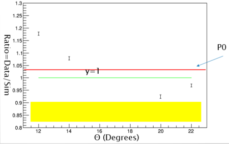
Shown above The r value is graphed with its respective theta (angle). The P0 line displays the line the points form. The line is very close to y=1 and within the error. The error bars represent the statistical error and error band the systematic. The r values are very close to one and the simulation is validated. It can now be used to make predictions for the kaon experiment.

Introduction

Since we validated the simulation we can now use it to predict the number of kaons we will detect from our kaon experiment. The experiment takes place next year. No experimental data has been collected yet. We hope to also determine the number of free pions (pions created during the kaon experiment) we should detect, and if there are enough pions created to study their form factor.

Input forms

Shown above are the values that will be used in the experiment at JLab next year. For this simulation we were detecting kaons.

SHMS

To detect Kaons we use the SHMS (Super High Momentum Spectrometer), which is new to JLab. The SHMS replaced the SOS spectrometer. The SHMS uses a similar PID set up to detect the particles that result from the reaction. Furthermore, we must apply cuts to out data to account for the SHMS acceptance.

SHMS Cuts

The cuts applied to the simulation's data inlclude the HMS acceptance and the SHMS acceptance. Shown below are the cuts from the SHMS. The HMS cuts follow the same procedure as shown previously when we validated the simulation. The ssdelta, ssxptar, and ssyptar represent the SHMS cuts. The SHMS cuts have the same definition as the HMS cuts, but are located on the SHMS Spectrometer. Shown below are the cuts applied to the 1.7 GeV run. The same cuts were applied to all of the other runs as well.

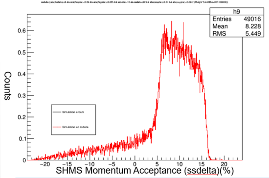
Graph 1:

Shown above is ssdelta data with and without the cut. The black line represents the data with the cuts applied -10% to 22%. The percentage is shown on the x axis. The data outside the cut would no be accepted by the spectrometer. The cuts allow for better prediction of what we expect to yield.

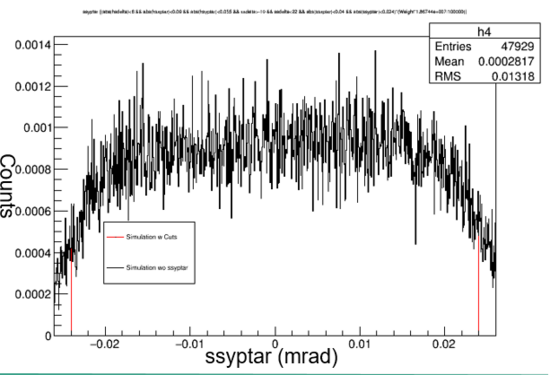
Graph 2:

Shown above is the ssyptar data with and without the cut. The acceptance is plus or minus 0.024 mrad and is graphed on the X-axis. Outside the acceptance would not be recorded by the spectrometer and with the cut it is not accepted by the simulation as well. The red line represents the data with cuts applied.

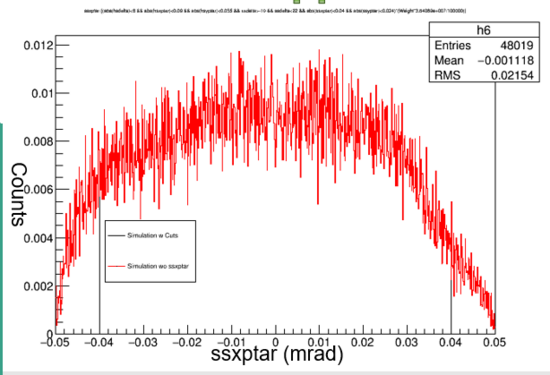
Graph 3:

Shown above is the ssxptar data with and without the cut. The acceptance is plus or minus 0.04 mrad and is graphed on the X-axis. Outside the acceptance would not be recorded by the spectrometer and with the cut it is not accepted by the simulation as well. The black line represents the data with cuts applied.

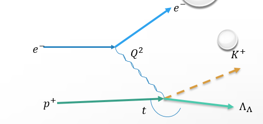
Fig 1:

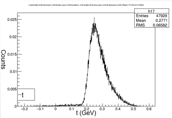
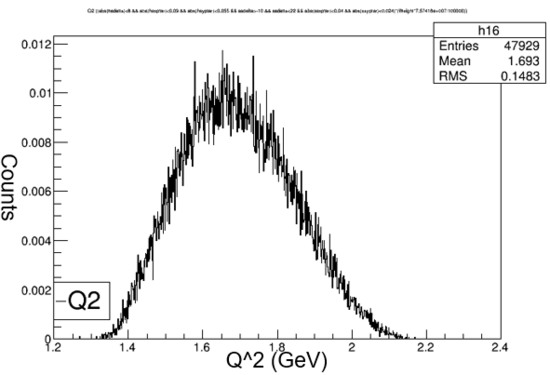
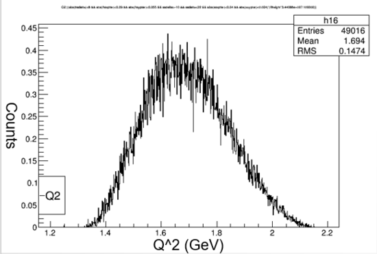
Shown above is a diagram showing the simplified Kaon reaction with the graphs of Q2 and t. Q2 represents the energy added by the electron to the reaction. t represents the energy added by the proton to the reaction. When the reaction occurs kaons are not the only particles created. Lambda represents the other particles that are needed in order to meet the conservation of momentum laws.

Graph 4:

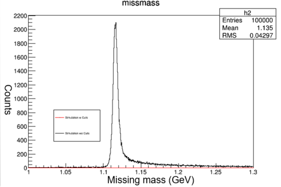
Shown above is the missing mass with all of the cuts applied (red line). The missing mass is graphed on the X-axis and counts on the Y-axis. The missing mass represents the mass needed in order to satisfy the conservation of momentum laws. It is the mass not detected by the spectrometer. Both the HMS and SHMS cuts are applied. The yield is very small, but when zoomed in a visible peak appears at 1.115 or the mass of Lambda. The lambda mass verifys that the simulation correctly produced the kaon electro production reaction because distribution should be centered on the Lambda mass (~1.115 GeV).

Calculations

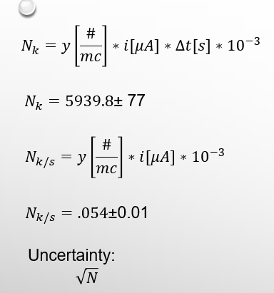
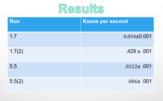
After completing the missing mass graph we completed the calculations to find the number of pions per second during each run. Shown below is the formula to find the number of pions per second. The yield is the area of the missmass graph with cuts applied. Then it is multiplied by the current and 10^3 to match the micro to milli. To find the total number of kaons then we would multiple by the run time, but since we want kaons per second we don't. The uncertainty is the square root of N (number of events). The experiment is set to run for several days. Even though it is a low amount, for the length of run time alot of kaons will be detected.

Shown below are the kaon per second numbers for the other runs.

Conclusion

Now that we have determined the number of Kaons produced we can figure out how many pions the experiment will produce. We can then determine whether enough are produced where we should detect them to study form factor. We can then determine the pion form factor uncertainty.

Pion Input Values

Next we programmed the simulation to detect pions. The simulation runs stayed the same, except now they detect pions instead of kaons. Shown below are the identical runs for detecting pions. In the code pion is now set to 1 to select it and kaon to 0 to deselect it. Only run 1.7 is shown below, however the same procedure was done for all of the other runs.

Cuts

All of the cuts and graphs were completed identical to the kaon analysis. Pions are also detected in the SHMS in which none of the acceptance changes only the particle being detected.

Missing Mass

The missing mass changes as shown in the diagram below.

Fig 1:

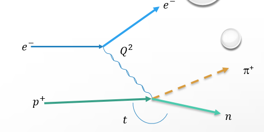
Shown above is a diagram showing the simplified pion reaction with the graphs of Q2 and t. Q2 represents the energy added by the electron to the reaction. t represents the energy added by the proton to the reaction. When the reaction occurs pions are not the only particles created. A neutron is also created and becomes the missing mass. The neutron allows the reaction to meet the conservation of momentum laws.

Graph 1:

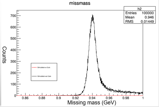
Shown above is the missing mass with all of the cuts applied (red line). The missing mass is graphed on the X-axis and counts on the Y-axis. The missing mass represents the mass needed in order to satisfy the conservation of momentum laws. It is the mass not detected by the spectrometer. Both the HMS and SHMS cuts are applied. The yield is very small, but when zoomed in a visible peak appears at 0.939 or the mass of a neutron. The neutron mass verifys that the simulation correctly produced the pion electro production reaction because the distribution (peak) should be centered on the neutron mass (~0.939 GeV). That mass correctly fulfills the conservation of momentum law.

Calculations

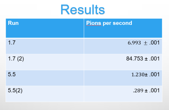
The calculations also remain the same as the kaon detection. The table below displays the number of pions per second for each run.

As the experiment is set to run for several days at each setting in which a very large amount of pions will be generated.

Pion Form Factor Uncertainty

Now that we know there will enough pions created to study we need to figure out the uncertainty of their form factor. THe pion form factor uncertainty is shown below.

Fig 2:

Delta sigma/sigma represents the combination of the systematic and statistical uncertainties. The statistical uncertainty is calculated through the square root of the number of pions created divided by the number of pions created for each trial. Epsilon 1 and 2 represent the epsilon values from the corresponding runs. The two .4s correspond as do the 1.7 and 5.5. Although the same epsilon values are used to calculate the uncertainty for the corresponding runs, the uncertainty is different because the statistical uncertainty is not the same. Each run has a different number of pions per second, hence a different number of total pions created.

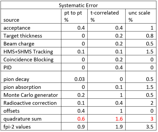
The systematic uncertainty is shown in the chart below.

Fig 3:

Shown above the quadrature sum or the red values were used as the systematic error in order to calculate the the pion form factor uncertainty.

Sample Calcs for the Pion Form Factor Uncertainty

Fig 4:

Shown below is step 1.

t correlated and stat unc are not included in this step to make sure they are not scaled by 1/change in epsilon.

Fig 5:

Step 2 is shown below.

Now the t correlated and stat unc are included in the calculation. This was repeated for each run as a different number of pions is produced fro each run.

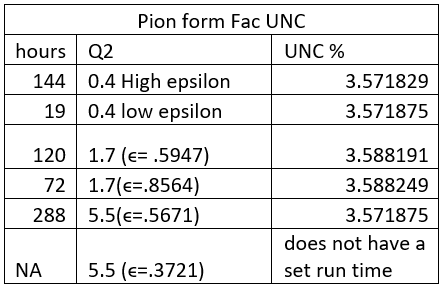
Below is a table displaying the pion form factor uncertainty for each run.

As seen above the uncertainty is rather low at around 3-4%. This means we have a very good chance at gaining insight into the pion form factor when the experiments occur next year.

Conclusion

As a result of the low pion form factor uncertainty we should optimize and make sure to detect pions while running the kaon experiment. Pion detection will give us insight into their form factor. Further research must be done to determine where and at what angle we will most likely detect pions.

Citations

Huber, G. M., G. J. Lolos, Z. Paoandreou, P. Bosted, A. Bruell, R. Ent, H. C. Fenker, D. Gaskell, T. Horn, M. K. Jones, D. Mack, D. Meekins, G. R. Smith, S. A. Wood, A. Asaturyan, A. Mkrtchyan, T. Navasardyan, V. Tadevosyan, D. Dutta, H. Gao, X. Qian, X. F. Zhu, W. Boeglin, P. Markowitz, J. Reinhold, E. Christy, C. E. Keppel, V. Tvaskis, E. Beise, H. Breuer, R. Gilman, J. Roche, W. Kim, S. S. Stepanyan, E. J. Brash, E. Gibson, D. Hornage, P. M. King, E. Korkmaz, A. K. Opper, I. Niculescu, C. F. Perdrisat, A. Sarty, and C. Xu. Jefferson Lab PAC 30 Proposal (n.d.): n. pag. Web.